Rust’s Nested Fixed Point Algorithm
Rust’s Nested Fixed Point Algorithm (NFXP)
본 포스트는 John Rust가 1987년 Econometrica에 게재한 Optimal Replacement of GMC Bus Engines: An Empirical Model of Harold Zurcher에 기반하여 만들어졌습니다.
1. Introduction
Rust는 Harold Zurcher라는 한 버스 정비 담당자의 버스 엔진 교체 행태를 설명하기 위한 regenerative optimal stopping 모델을 제안했습니다. Rust의 귀무가설은 “Zurcher가 매 순간 버스 엔진을 교체할지 말지 결정하는 데 있어 regenerative optimal stopping rule을 따른다”인데, 여기서 optimal stopping rule은 분석가들이 관찰하거나(예. 주행거리) 혹은 관찰할 수 없는 여러 state variable들로 구성된 함수일 것입니다. 한편, 이름에 regenerative가 들어가는 이유는 엔진을 교체할 경우 주행거리를 중심으로 한 일부 state들이 초기화되기 때문이고요.
만약 Zurcher가 지금 당장 엔진을 교체한다면 즉각적으로 교체 비용이 발생할 것이고, 교체하지 않는다면 언제일지 모르는 미래에 버스가 고장나서 예상치 못한 비용을 지불해야 할 수 있습니다. 따라서 각 시점마다 엔진을 교체할 때와 교체하지 않을 때 발생 가능한 비용 중 최소 비용을 부담하기 위한 선택이 내려질 것이고, 이에 대한 optimal stopping rule은 stochastic dynamic programming 문제의 solution으로 표현 가능합니다.
Stochastic dynamic programming 문제를 풀기 위한 Rust의 nested fixed point algorithm은 likelihood function $L(\theta)$를 극대화하는 $\theta$를 찾는 “outer” optimization algorithm과 주어진 $\theta$ 값에 대하여 fixed point $EV_{\theta}$를 계산하는 “inner” fixed point algorithm 등 두 개의 알고리즘이 중첩된 형태로 구성됩니다.
2. Model
시점 $t$까지 적립된 버스의 주행거리를 $x_t$라는 관찰 가능한 state variable로 생각해 봅시다. 그리고 시점 $t$마다 Zurcher의 엔진 교체 결정은 0 또는 1의 값을 가지는 $d_t$로 표기하겠습니다. $d_t$가 0이면 엔진을 유지하는 결정이고, 1이면 새로운 엔진으로 교체하는 결정입니다.
각 시점 $t$마다 Zurcher가 예상하는 비용인 expected per period costs는 $x_t$에 대해 증가하고 미분 가능한 함수 $c(x_t,\theta)$라고 가정하겠습니다. $c(x_t,\theta)$에는 엔진 교체에 필요한 인력 비용과 같이 직접적으로 관찰할 수 있는 비용뿐만 아니라 직접 관찰할 수는 없지만 엔진을 교체하지 않았을 때 예기치 못한 고장으로 인해 발생 가능한 비용에 대한 Zurcher의 전망치도 함께 포함될 것입니다.
한편, Zurcher는 의사결정 시 관찰할 수 있지만 우리 분석가들은 관찰할 수 없는 state variable들도 분명 있을 것입니다. Rust는 이러한 unobserved state variable들을 각 선택 $d_{t}$에 대하여 $\epsilon_t = { \epsilon_t{(0)}, \epsilon_t{(1)} }$로 표기했습니다.
종합적으로 시점 $t$에 state variables $x_t$와 $\epsilon_t$가 주어지고, Zurcher가 비용 함수 $c(x_t,\theta)$를 가지며, 엔진을 교체할지 유지할지에 대한 선택 $d_t$를 결정할 때, single period utility function $u(x_t,d_t,\theta) + \epsilon_t(d_t)$를 예를 들어 아래와 같이 정의할 수 있을 것입니다.
\[\begin{equation} u(x_t,d_t,\theta) + \epsilon_t(d_t) = \begin{cases} -RC - c(0,\theta) + \epsilon_t(1) & \text{if } d_t=1 \\ -c(x_t,\theta) + \epsilon_t(0) & \text{if } d_t=0 \end{cases} \end{equation}\]State variable들은 Markov process를 따르는데, 이때 transition density가 $\pi(x_{t+1},\epsilon_{t+1} \vert x_t,\epsilon_t,d_t,\theta)$로 주어진다고 가정해 봅시다. 나아가 문제를 쉽고 풀 수 있게 만들기 위해서 Rust는 아래와 같이 Conditional Independence (CI) Assumption이라는 또 하나의 중요한 가정을 제안합니다.
\[\begin{equation} \pi(x_{t+1},\epsilon_{t+1} | x_t,\epsilon_t,d_t,\theta) = p(x_{t+1} | x_t,d_t,\theta) q(\epsilon_t | x_t,\theta) \end{equation}\] \[\begin{equation} p(x_{t+1} | x_t,d_t,\theta) = \begin{cases} g(x_{t+1}-0 | \theta) & \text{if } d=1 \\ g(x_{t+1}-x_t | \theta) & \text{if } d=0 \end{cases} \end{equation}\]Stationary infinite horizon case에서 optimal value function $V_{\theta}$는 아래 Bellman equation의 unique solution입니다. 현 시점의 utility value를 제외하고 미래에 대한 기대에 해당하는 마지막 항을 expected value function $EV_{\theta}$와 discount factor $\beta$의 곱으로 좀더 간단히 표기하겠습니다.
\[\begin{equation} \begin{split} V_{\theta}(x,\epsilon) &= \max_{d \in D(x)} {[u(x,d,\theta) + \epsilon(d) + \beta \int{V_{\theta}(x',\epsilon') \pi(dx',d\epsilon' | x,\epsilon,d,\theta)}]} \\ &= \max_{d \in D(x)} {[u(x,d,\theta) + \epsilon(d) + \beta EV_{\theta}(x,\epsilon,d)]} \end{split} \end{equation}\]CI 가정 덕분에 likelihood function $L(\theta)$를 아래와 같이 정의할 수 있습니다.
\[\begin{equation} L(\theta) = \prod_{t=2}^{T} {P(d_t | x_t,\theta) p(x_t | x_{t-1},d_{t-1},\theta)} \end{equation}\]conditional choice probability $P(d \vert x,\theta)$는 우리가 잘 아는 multinomial logit 공식을 통해 표현됩니다.
\[\begin{equation} P(d | x,\theta) = \frac{ \exp{\{ u(x,d,\theta) + \beta EV_{\theta}(x,d) \}} } { \sum_{d' \in D(x)}{ \exp{\{ u(x,d',\theta) + \beta EV_{\theta}(x,d') \}} } } \end{equation}\]Contraction mapping
\[\begin{equation} \begin{split} EV_{\theta}(x,d) &= T_{\theta}(EV_{\theta}(x,d)) \\ &= \int{\log{[ \sum_{d' \in D(x')}{\exp{\{ u(x',d',\theta) + \beta EV_{\theta}(x',d') \}}} ] p(dx'|x,d,\theta)}} \end{split} \end{equation}\]3. NFXP Algorithm
3.1. “Inner” Fixed Point Polyalgorithm
3.2. “Outer” BHHH Optimization Algorithm
BHHH 알고리즘에서 파라미터 업데이트는 다음과 같이 진행됩니다.
\[\begin{equation} \theta_{k+1} = \theta_{k} + \lambda D(\theta_{k}) \end{equation}\]만약 $\lambda=1$이고 $D(\theta)$가 아래와 같이 주어질 때 BHHH는 Newton’s method와 동일해집니다.
\[\begin{equation} D(\theta) = -[\partial^2{L(\theta)} / \partial{\theta}\partial{\theta'}]^{-1} \partial{L(\theta)} / \partial{\theta} \end{equation}\]4. Data
Ref: https://github.com/OpenSourceEconomics/rust-data
import numpy as np
import pandas as pd
import matplotlib.pyplot as plt
# raw data 읽어오기
g1 = np.loadtxt("./assets/05-NFXP/data/g870.asc").reshape(15,36)
g2 = np.loadtxt("./assets/05-NFXP/data/rt50.asc").reshape(4,60)
g3 = np.loadtxt("./assets/05-NFXP/data/t8h203.asc").reshape(48,81)
g4 = np.loadtxt("./assets/05-NFXP/data/a530875.asc").reshape(37,128)
g5 = np.loadtxt("./assets/05-NFXP/data/a530874.asc").reshape(12,137)
g6 = np.loadtxt("./assets/05-NFXP/data/a452374.asc").reshape(10,137)
g7 = np.loadtxt("./assets/05-NFXP/data/a530872.asc").reshape(18,137)
g8 = np.loadtxt("./assets/05-NFXP/data/a452372.asc").reshape(18,137)
data = None

g_id = 1
for g in [g1,g2,g3,g4,g5,g6,g7,g8]:
# for g in [g5]:
    # 헤더: 버스 ID, 구매 일자, 교체 시점 및 odometer readings, 최초 관측 일자 (일자들은 연/월 구분)
    head = pd.DataFrame(g[:,:11], columns=["id","purc_m","purc_y",
                                            "repl_1_m","repl_1_y","repl_1_odo",
                                            "repl_2_m","repl_2_y","repl_2_odo",
                                            "begin_m","begin_y"]).astype(int)

    # ym: year-month pairs
    y, m = int(head.begin_y.unique()), int(head.begin_m.unique())-1
    ym = []
    for i in range(pd.DataFrame(g[:,11:]).shape[1]):
        if m ==12:
            y += 1
            m = 1
        else:
            m += 1
        ym.append(str(y)+"-"+str(m))

    # 본문: 버스-일자-레벨 패널 데이터 생성
    g_ref = pd.DataFrame(g[:,11:], index=g[:,0].astype(int), columns=ym).stack().reset_index()
    g_ref.columns = ["id","date","odo"]
    g_ref.insert(loc=0, column="group", value=g_id) # 그룹 ID

    # 헤더 정보와 패널로 변환한 본문 결합
    head["date_begin"] = head.apply(lambda row: str(row["begin_y"])+"-"+str(row["begin_m"]), axis=1)
    g_ref = pd.merge(g_ref, head[["id","date_begin"]], how="left") #### maybe ignorable

    head["date"] = head.apply(lambda row: str(row["repl_1_y"])+"-"+str(row["repl_1_m"]), axis=1)
    repl_1 = head[["id","date","repl_1_odo"]].query("repl_1_odo != 0")
    g_ref = pd.merge(g_ref, repl_1, how="left")

    head["date"] = head.apply(lambda row: str(row["repl_2_y"])+"-"+str(row["repl_2_m"]), axis=1)
    repl_2 = head[["id","date","repl_2_odo"]].query("repl_2_odo != 0")
    g_ref = pd.merge(g_ref, repl_2, how="left")

    # 종속변수 repl: 엔진 교체 여부 (0 또는 1)
    g_ref["repl"] = g_ref.apply(lambda row: 1 if row["repl_1_odo"]==row["repl_1_odo"] or row["repl_2_odo"]==row["repl_2_odo"] \
                                else 0, axis=1)
    g_ref["repl_cum"] = g_ref.groupby("id").repl.cumsum()

    p_list = []
    for b_id, b in g_ref.groupby("id")["repl"]:
        p = 1
        for d in b:
            if d == 0:
                p_list.append(p)
                p += 1
            else:
                p_list.append(p)
                p = 0
    g_ref["period"] = p_list

    # 설명변수 mileage: mileage at replacement
    tmp = g_ref.groupby("id").repl_1_odo.max().to_frame("odo_1").reset_index()
    g_ref = pd.merge(g_ref, tmp, how="outer")
    tmp = g_ref.groupby("id").repl_2_odo.max().to_frame("odo_2").reset_index()
    g_ref = pd.merge(g_ref, tmp, how="outer")

    def x_ref(row):
        if row["repl"]==1 and row["repl_cum"]==1:
            return row["repl_1_odo"]
        elif row["repl"]==1 and row["repl_cum"]==2:
            return row["repl_2_odo"] - row["odo_1"]
        elif row["repl"]==0 and row["repl_cum"]==0:
            return row["odo"]
        elif row["repl"]==0 and row["repl_cum"]==1:
            return row["odo"] - row["odo_1"]
        elif row["repl"]==0 and row["repl_cum"]==2:
            return row["odo"] - row["odo_2"]
    g_ref["mileage"] = g_ref.apply(x_ref, axis=1)

    # 불필요한 변수 제거
    g_ref.drop(columns=["odo","repl_1_odo","repl_2_odo","repl_cum","odo_1","odo_2","date_begin"], inplace=True)

    # concat
    if data is None:
        data = g_ref
    else:
        data = pd.concat([data, g_ref]).reset_index(drop=True)

    g_id += 1

data
| group | id | date | repl | period | mileage | |
|---|---|---|---|---|---|---|
| 0 | 1 | 4403 | 83-5 | 0 | 1 | 504.0 |
| 1 | 1 | 4403 | 83-6 | 0 | 2 | 2705.0 |
| 2 | 1 | 4403 | 83-7 | 0 | 3 | 7345.0 |
| 3 | 1 | 4403 | 83-8 | 0 | 4 | 11591.0 |
| 4 | 1 | 4403 | 83-9 | 0 | 5 | 16057.0 |
| ... | ... | ... | ... | ... | ... | ... |
| 15563 | 8 | 4256 | 85-1 | 0 | 87 | 138474.0 |
| 15564 | 8 | 4256 | 85-2 | 0 | 88 | 139320.0 |
| 15565 | 8 | 4256 | 85-3 | 0 | 89 | 140616.0 |
| 15566 | 8 | 4256 | 85-4 | 0 | 90 | 141292.0 |
| 15567 | 8 | 4256 | 85-5 | 0 | 91 | 142426.0 |
15568 rows × 6 columns
# Table 2a
display(np.round(data.query("repl==1").groupby("group").mileage.describe()))
display(np.round(data.query("repl==1").groupby("group").period.describe(),1))
| count | mean | std | min | 25% | 50% | 75% | max | |
|---|---|---|---|---|---|---|---|---|
| group | ||||||||
| 3 | 27.0 | 199733.0 | 37459.0 | 124800.0 | 174550.0 | 204800.0 | 230650.0 | 273400.0 |
| 4 | 33.0 | 257336.0 | 65477.0 | 121300.0 | 215000.0 | 264100.0 | 292400.0 | 387300.0 |
| 5 | 11.0 | 245291.0 | 60258.0 | 118000.0 | 229600.0 | 250600.0 | 282250.0 | 322500.0 |
| 6 | 7.0 | 150786.0 | 61007.0 | 82400.0 | 107450.0 | 125500.0 | 197750.0 | 237200.0 |
| 7 | 27.0 | 208963.0 | 48981.0 | 121000.0 | 178650.0 | 207700.0 | 237200.0 | 331800.0 |
| 8 | 19.0 | 186700.0 | 43956.0 | 132000.0 | 162900.0 | 182100.0 | 188400.0 | 297500.0 |
| count | mean | std | min | 25% | 50% | 75% | max | |
|---|---|---|---|---|---|---|---|---|
| group | ||||||||
| 3 | 27.0 | 54.1 | 10.9 | 33.0 | 45.5 | 56.0 | 63.5 | 69.0 |
| 4 | 33.0 | 72.6 | 23.3 | 27.0 | 53.0 | 76.0 | 86.0 | 115.0 |
| 5 | 11.0 | 82.5 | 29.8 | 29.0 | 73.0 | 82.0 | 99.5 | 126.0 |
| 6 | 7.0 | 72.1 | 34.7 | 47.0 | 47.0 | 51.0 | 95.0 | 123.0 |
| 7 | 27.0 | 47.0 | 27.6 | 10.0 | 28.5 | 39.0 | 66.5 | 102.0 |
| 8 | 19.0 | 26.1 | 25.9 | 2.0 | 7.0 | 16.0 | 37.0 | 91.0 |
# Table 2b
bus_nr = data.groupby("id").repl.sum()
bus_nr = bus_nr[bus_nr == 0].index
display(np.round(data[data.id.isin(bus_nr)].groupby(["group","id"]).last().mileage.groupby("group").describe()))
display(np.round(data[data.id.isin(bus_nr)].groupby(["group","id"]).last().period.groupby("group").describe(),1))
| count | mean | std | min | 25% | 50% | 75% | max | |
|---|---|---|---|---|---|---|---|---|
| group | ||||||||
| 1 | 15.0 | 100117.0 | 12929.0 | 65643.0 | 98580.0 | 101423.0 | 106280.0 | 120151.0 |
| 2 | 4.0 | 151182.0 | 8530.0 | 142009.0 | 145907.0 | 150486.0 | 155762.0 | 161748.0 |
| 3 | 21.0 | 250766.0 | 21325.0 | 199626.0 | 244599.0 | 254183.0 | 267988.0 | 280802.0 |
| 4 | 5.0 | 337222.0 | 17802.0 | 310910.0 | 326724.0 | 347549.0 | 348475.0 | 352450.0 |
| 5 | 1.0 | 326843.0 | NaN | 326843.0 | 326843.0 | 326843.0 | 326843.0 | 326843.0 |
| 6 | 3.0 | 265264.0 | 33332.0 | 232395.0 | 248376.0 | 264356.0 | 281698.0 | 299040.0 |
| count | mean | std | min | 25% | 50% | 75% | max | |
|---|---|---|---|---|---|---|---|---|
| group | ||||||||
| 1 | 15.0 | 25.0 | 0.0 | 25.0 | 25.0 | 25.0 | 25.0 | 25.0 |
| 2 | 4.0 | 49.0 | 0.0 | 49.0 | 49.0 | 49.0 | 49.0 | 49.0 |
| 3 | 21.0 | 70.0 | 0.0 | 70.0 | 70.0 | 70.0 | 70.0 | 70.0 |
| 4 | 5.0 | 117.0 | 0.0 | 117.0 | 117.0 | 117.0 | 117.0 | 117.0 |
| 5 | 1.0 | 126.0 | NaN | 126.0 | 126.0 | 126.0 | 126.0 | 126.0 |
| 6 | 3.0 | 126.0 | 0.0 | 126.0 | 126.0 | 126.0 | 126.0 | 126.0 |
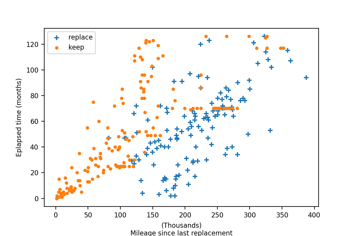
# Figure 1
plt.rcParams["figure.dpi"] = 100
plt.rcParams["figure.figsize"] = (6,4)
plt.rcParams.update({'font.size': 8})
fig = plt.figure()
ax = fig.add_subplot(111)

g_repl = data[data.repl==1].reset_index(drop=True)
g_main = data[data.repl==0].groupby("id").last().reset_index(drop=True)

g_repl.mileage = g_repl.mileage / 1000
g_main.mileage = g_main.mileage / 1000

ax.scatter(g_repl["mileage"], g_repl["period"], label="replace", marker="+")
ax.scatter(g_main["mileage"], g_main["period"], label="keep", s=10)

plt.ylabel("Eplapsed time (months)")
plt.xlabel("(Thousands)\nMileage since last replacement")
plt.legend()
plt.savefig("./assets/05-NFXP/nfxp_01.png", dpi=200)